


Resampling digitized audio
We have seen how to reduce the size of the digitized guitar string sound, to make it fit into the microcontroller Flash memory.
Reproducing the original sound at the same frequency is easy: it just requires feeding the digitized values to a DAC at the same sampling rate used for recording.
If you followed these posts, you will remember that a PWM can be used as a DAC to convert a sequence of digital values to an analog audio signal. There are a few catches, but I will write about them later.
My original digitized sound was a G (Sol) musical note from the third string of a guitar (196 Hz), so playing it back will produce the same G note.
But a single-note instrument would be quite boring. How could I produce a different note, for example a D (Re) that has a frequency of 293.7 Hz?
This D is a musical ‘fifth’ above the original G; its frequency is almost exactly 1.5 times the original frequency. I chose a D because 1.5x is good for illustration, but what follows works equally well for any desired note (within limits).
The naive way
First, to avoid confusion:
Sampling rate: the digitizing (recording) frequency, i.e. the rate at which the istantaneous wave values were read into numeric samples.
Playing rate: the frequency at which the numeric sampled values are sent to the DAC for playing.
A simple way to play back our wave at 1.5x the frequency could be to send the sampled values to the DAC faster than they were recorded, that is to use a playing rate higher than the original sampling rate.
To get the desired D note, that has 1.5 times the frequency of our original G note, the samples should be sent at 1.5x the sampling rate:
Sampling frequency = 44100 Hz
Playing rate = 44100 Hz * 1.5 = 66150 Hz
This would work, but unfortunately it has unintended consequences because the playing rate would vary from note to note.
It would be quite difficult, or plainly impossible, to design the analog filter, because such a filter has to be designed for a well defined frequency (more on the filter later).
The hardware could be unable to reproduce the samples at the required range of different frequencies: the highest note on a guitar has a frequency that is about 12 times that of the lowest note. Also, the hardware could work better at a fixed frequency.
Lowering the playing rate could produce audible undesired frequencies (artefacts), causing ‘intermodulation distortion’.
There is a better way, even if it is not perfect.
Resampling
Instead of using the original sampled values and playing them out at a rate depending on the desired note, we can do the opposite: compute a new list of sampled values for the desired note frequency.
If played at a sampling rate equal to the original sampling rate, this new list of samples will sound as a wave of a different frequency.
Computing a new list of samples from an existing list is called resampling. Let us see how it works in our case.
The image below shows a cycle of a sine wave (a ‘pure’ waveform) sampled at regular intervals.
The red lines represent the sampling times, the height of each blue dot is the corresponding sampled value, stored as a number (we have already seen this).
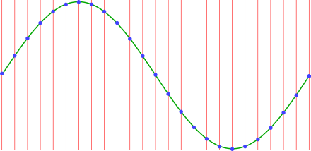
After digitizing it, all that remains of the original wave are the sampled values (the blue dots). However, I will continue drawing the original wave as a visual reference.
Change the time, keep the time
To play this wave at a frequency higher than the original, we can use samples taken farther apart on the original wave.
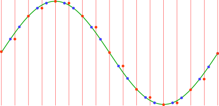
To play the wave at 1.5x the original frequency, imagine re-reading the (sampled) wave values at 1.5 times the original time interval. I am not referring to the original sampling rate, but to the list of numeric values (the samples).
The points where the red lines here cross the wave represent the new (imaginary) re-sampling points:

But we do not have all these points, so we use the value of the preceding sampling point when a real point (blue dot) is not available.
(it would be much better to linearly interpolate between blue points, but this would cost too much on an 8-bit microcontroller, especially when playing many voices)
The red dots here are the new, resampled values, that is the values we will actually send to the DAC:
Now we take the red dot values and play them out (using the DAC) using the original sampling rate as playing rate. We have produced a wave with 1.5x the original frequency:

As you can see, in the same number of samples as one cycle of the original wave, i.e in the same time because we are using the same playing rate, we play 1.5 wave cycles. So we are playing at 1.5 times the original frequency: a D instead of the original G.
This operation is usually done on the fly, without any precalculation. I will later show some AVR code.
Actually, it is not necessary for the playing rate to be the same as the sampling frequency (in fact, in play-v6 it is not). What really counts to avoid the problems I mentioned above in “The naive way” is that the playing rate is the same for all notes.
The ugly truth
Doesn’t the above resampled wave look nice?
Well, let us remove the nice sine wave drawing and connect the red dots to see how the DAC output will actually look:
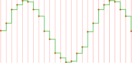
Urgh! Here the lack of interpolation is quite visible as wave asymmetry. Such a sound will surely be totally unacceptable!
Well, actually it could sound pleasant enough. The trick is to have enough sampling points in the original wave to avoid gross distortion, so the original wave should be digitized at the highest possible sampling rate.
That’s why I preferred to shorten the guitar sound, rather than reducing its sampling rate.
So, to recap, we have a sampled guitar string sound and we know (at least in theory) how to play it at different rates to produce different notes.
I previously wrote that optimization is the art of finding the best compromise between conflicting requirements, so in the next post I will consider another set of conflicting requirements.