


Hibernation
This blog is currently in deep sleep, please do not make loud noises.
A long silence, I know…
I am rather overloaded on the work side, and no relief in sight. Thanks for the patience :-)
An earlier play-v6 version
I started working on play-v6 in the first days of December 2013 and in about three weeks I could play “Jingle Bells”: in time for Christmas :-)
That early version (450 git commits ago) had lots of limitations but reproduced my sampled guitar string sound on six voices.
My test actually used three voices:
Let us see how a voice was played.
The guitar sound in memory
The guitar string sound exported from Audacity was stored in a constant byte array in the code:
PROGMEM const int8_t samples[] = {
0xff, 0xff, 0xff, 0xff, 0xff, 0xff, 0xff, 0xff, 0xff, 0xff, 0xff, 0xff,
0xff, 0x00, 0x00, 0x00, 0x00, 0x00, 0x00, 0x00, 0x00, 0x00, 0x00, 0x00,
0x00, 0x00, 0x00, 0x00, 0x00, 0x00, 0x00, 0x00, 0x00, 0x00, 0x00, 0x00,

// [ ... ]

0xdf, 0xdb, 0xd8, 0xd5, 0xd2, 0xcf, 0xcc, 0xc9, 0xc5, 0xc3, 0xc0, 0xbd,
0xba, 0xb8, 0xb5, 0xb3, 0xb2, 0xb0, 0xaf, 0xae, 0xad, 0xad, 0xac, 0xab,
0xa9, 0xa9, 0xa7, 0xa6, 0xa6, 0xa6, 0xa6, 0xa7, 0xa7, 0xa8, 0xa9, 0xab,
0xad, 0xae, 0xb0, 0xb2, 0xb5, 0xb8, 0xbb, 0xbe, 0xc1, 0xc4, 0xc6, 0xc9,
0xcb, 0xcd, 0xcf, 0xd2, 0xd5, 0xd8, 0xdb, 0xde, 0xe2, 0xe5, 0xe8, 0xec,
0xef, 0xf3, 0xf6, 0xf9, 0xfd, 0x01, 0x05, 0x08, 0x0b, 0x0e, 0x10, 0x12,

// [ ... ]

};
The PROGMEM directive tells the compiler to store these data into the Flash memory and to avoid copying them to RAM at startup (there would be no space for them!)
This creates a small complication, because AVR microcontrollers use the Harvard architecture: data and code have separate memory addressing spaces. It means that the above sampled audio data cannot be accessed with normal instructions.
A fixed-point voice pointer
You may remember the theory about how to play a digitized sound at a different frequency. Here is an actual implementation from my early player.
This structure represents the playing status of a voice:
//status of a single voice, will point to wave samples in PROGMEM
typedef struct Voice
{
const int8_t   *wavePtr;        //current position (16.8)
uint8_t         wavePtrFrac;    //(no need for alignment padding, access is 8-bit)
const int8_t   *loopHere;       //loop back a PWM_CYCLE when wavePtr gets past this point
uint16_t        waveStep;       //wavePtr advance step (8.8), determines pitch
} Voice;
(sorry for the limited width; I know this blog format is not well suited to code listings, but I am a guest here)
The most interesting thing here is the 16.8 pointer. What does that mean?
To resample while playing, we need to use a fractional increment for the pointer into the sampled sound data; in this case I used 16 bits of integer part (wavePtr) and 8 bits of fractional part (wavePtrFrac).
In other terms, the integer part points to the actual sample into the data (we cannot read between the data!) while the fractional part keeps track of the residual fraction that will be added on the next step.
The speed at which the sampled data is read is determined by another fractional value, this time with 8 bits of integer part and 8 bits of fractional part: waveStep. In short:
wavePtr = wavePtr + waveStep
using fixed-point values in 16.8 format.
Playing out a voice
C does not offer 24-bit fixed-point arithmetic, so it must be built using existing instructions (I could use 32-bit operations, but that would be horribly inefficient on an 8-bit processor).
To get the current sample for a voice, I use the pseudo-function call pgm_read_byte_near() to get from the sampled data array in Flash memory the value pointed by wavePtr:
//get current sample
sample = pgm_read_byte_near(vp->wavePtr);
Then I advance the 16.8 pointer by the fractionary 8.8 step(that determines the frequency (i.e. the musical note being played) and keep the 0.8 fractional rest:
//advance to next sample (16.8 wavePtr + 8.8 waveStep):
//first add .8 fractional remainder from previous cycle to get 8.8 step
step = (uint16_t)vp->wavePtrFrac + vp->waveStep; //(0.8 + 8.8, no overflow)
//keep .8 for next cycle
vp->wavePtrFrac = step & 0xff;
//add 8. to wave pointer (16. + 8.)
vp->wavePtr += (step >> 8); //(logical shift is ok: step bit 15 is 0)
Last, I check for the end of the data array (the end of the guitar string sound) and, in that case, continue to play the same note. That is done to prolong the trailing string sound that I had to cut short for lack of memory space.
</pre>
//if end reached, enter 1-cycle loop
if (vp->wavePtr >= vp->loopHere)
{
vp->wavePtr -= WAVE_CYCLE;
}
WAVE_CYCLE is the number of samples making up a single cycle of the digitized wave. In practice, it continues to play the same cycle.
The sum of six voices
When I had the six ‘sample’ values for the six voices, my first idea was to add them up and send the result to a single PWM output (working as DAC). But I had a problem.
Each 8-bit voice can have 256 possible values, so the sum of six voices can have:
256 * 6 = 1536 possible values
If I wanted to use a PWM, I needed a timer that could count from 0 to 1535. No problem here: the timer 1 on the ATmega368P can count up to 65535.
If you remember the previous post, you may have guessed where my problem was.
The timer cannot count faster than the CPU clock, that is 16 MHz. So the PWM frequency, the maximum rate at which I could play the digitized samples, would have been:
16 MHz / 1536 = ~10417 Hz
Alas, 10.4 kHz is well within the audible range: a loud high-pitched sound would be audible. Filtering it out without cutting off some of the music ‘brillance’ would be quite problematic (more about filters in a future post).
Raising the PWM frequency
A better idea would have been to double the PWM frequency, using 768 possible values instead of 1526:
16 MHz / 768 = ~20833 Hz
A 20 kHz signal is easier to filter out without disturbing the music too much (we are not talking Hi-Fi here). But 768 possible values are not enough for six 8-bit voices!
I could have added the six values up and then thrown away the least significant bit (i.e. divided the result by 2)
(256 * 6) / 2 = 768 possible values
The first compromise
Actually, I initially decided for a different approach to get a bit more time for computations and a bit more quality: I set a PWM frequency of about 16 kHz, using 1024 (10 bits) as PWM count.
Then I reduced the volume of the sampled sound from 256 to 170 possibles value, so that the sum of the six voices could not exceed 1024:
1024 / 6 = 170 (discarding the fractional part)
It worked, as you can hear from the audio clip at the start of this post, but my son said:
“Dad, can you take out that whistling sound?”
Despite my filter, the 16 kHz from the PWM output was still audible. I could not hear it, but he could.
It was the start of a long optimization voyage… but that is another story.
New toy
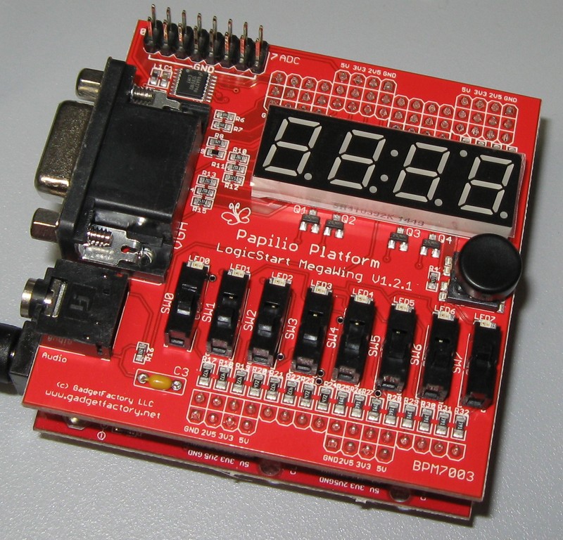
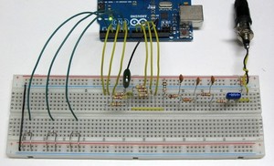
It is programmable but it does not (usually) run a program: it is an FPGA evaluation and learning board.
For lazy designers like myself, it beats building circuit prototypes the way I used to… ‘some’ time ago:

This video card (1979) was part of our industrial modular system and stayed in production for many years. Not in this form ;-)
Most of the ICs with white stick-on labels in the above prototype were ancestors of modern FPGA devices; they were called PALs.
Bit depth, PWM and frequency
I have briefly shown how to resample a digital audio recording to play it out at a different pitch (i.e. at a different frequency).
Using PWM (pulse-width modulation) as a form of DAC (digital to analog converter) introduces some additional constraints we must be aware of when designing a player.
As we have seen, inside a microcontroller (such as the ATmega328P used in the Arduino Uno) a PWM is typically implemented in hardware using a timer that counts up from zero to a maximum value (e.g. 255) and a comparator that checks when it is time to turn the output off.
If we use an 8-bit counter for the PWM and let it count to the maximum, it has 28 = 256 possible values. With an 8-bit counter we will not be able to use more then 8 bits for each audio sample, that is 8 bits of audio bit depth (resolution), but that was expected.
PWM resolution, timer clock and playing rate
It may be less obvious that the PWM resolution also sets a limit on the playing rate, i.e. the frequency we are using to play out the audio sampled values.
That happens because counting from zero to the maximum value (e.g. 255 for an 8-bit timer) takes time. An 8-bit timer requires 256 input (clock) pulses for a full count:
Playing_rate = timer_clock / 256
The timer clock frequency is usually selectable. In the case of the ATmega328P (Arduino Uno) the highest possible value is the same as the CPU clock: 16 MHz.
So the maximum playing rate for an 8-bit PWM DAC is:
Playing_rate = 16000000 Hz / 256 = 62500 Hz
62.5 kHz are plenty enough for audio, even considering that, to prevent undesired audible artifacts, the playing rate should be at least double the highest audio frequency we intend to play (I am skipping many subtle points here, especially because we are dealing with digitized audio, but this is the most important requirement).
So, no problems? Not so fast.
The cost of code
Getting the next sampled value from the original digitized wave and writing it into the PWM counter takes time, especially considering that a resampling is needed to output the desired audio frequency.
From a sample to the next, assuming the above 62.5 kHz, there are 256 CPU clock cycles available; they should be more than enough to do the necessary computations an other operations.
But…
…did I mention that I wanted to play six independent voices? The number of clock cycles available for each voice becomes:
256 clock cycles / 6 = 42 clock cycles
That is not easy to achieve using “casual C”. It requires a fair bit of optimization, including looking at the code produced by the compiler to see where precious CPU cycles could be saved.
Oh, I forgot: there is also the music score to read for each voice, the note duration to control, possibly also the note volume!
Forget the 256 cycles. A more realistic objective could be to do it all in 512 cycles. In that case:
Playing_rate = 16000000 Hz / 512 = 31250 Hz
31.25 kHz is still good. In fact, it took many iterations and a lot of work to get there, as I will show in the following posts.
From Audacity to 8-bit data
Before (finally!) talking about actual code, recall that my sampled guitar string had to be saved as 8 bits per sample to fit into the available microcontroller Flash memory.
This can be done in Audacity choosing File -> Export Audio… and selecting Other uncompressed files:
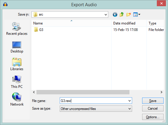
then pressing the Options… button and selecting RAW and Signed 8 bit PCM:
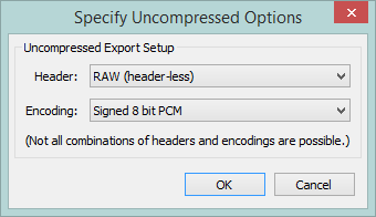
“RAW” means to save just the audio samples, devoid on any extra information such as the header that in the common audio formats (e.g. .wav) contains information about the samples.
“Signed” means that the value of each sample will go from -128 to +127, not from 0 to 255. The zero value will correspond to the central line (silence); applying volume and summing waves together will be easier and faster.
That’s all for the theory (at least for now…). In the next post: some code from my first ‘real’ player.
Resampling digitized audio
We have seen how to reduce the size of the digitized guitar string sound, to make it fit into the microcontroller Flash memory.
Reproducing the original sound at the same frequency is easy: it just requires feeding the digitized values to a DAC at the same sampling rate used for recording.
If you followed these posts, you will remember that a PWM can be used as a DAC to convert a sequence of digital values to an analog audio signal. There are a few catches, but I will write about them later.
My original digitized sound was a G (Sol) musical note from the third string of a guitar (196 Hz), so playing it back will produce the same G note.
But a single-note instrument would be quite boring. How could I produce a different note, for example a D (Re) that has a frequency of 293.7 Hz?
This D is a musical ‘fifth’ above the original G; its frequency is almost exactly 1.5 times the original frequency. I chose a D because 1.5x is good for illustration, but what follows works equally well for any desired note (within limits).
The naive way
First, to avoid confusion:
Sampling rate: the digitizing (recording) frequency, i.e. the rate at which the istantaneous wave values were read into numeric samples.
Playing rate: the frequency at which the numeric sampled values are sent to the DAC for playing.
A simple way to play back our wave at 1.5x the frequency could be to send the sampled values to the DAC faster than they were recorded, that is to use a playing rate higher than the original sampling rate.
To get the desired D note, that has 1.5 times the frequency of our original G note, the samples should be sent at 1.5x the sampling rate:
Sampling frequency = 44100 Hz
Playing rate = 44100 Hz * 1.5 = 66150 Hz
This would work, but unfortunately it has unintended consequences because the playing rate would vary from note to note.
It would be quite difficult, or plainly impossible, to design the analog filter, because such a filter has to be designed for a well defined frequency (more on the filter later).
The hardware could be unable to reproduce the samples at the required range of different frequencies: the highest note on a guitar has a frequency that is about 12 times that of the lowest note. Also, the hardware could work better at a fixed frequency.
Lowering the playing rate could produce audible undesired frequencies (artefacts), causing ‘intermodulation distortion’.
There is a better way, even if it is not perfect.
Resampling
Instead of using the original sampled values and playing them out at a rate depending on the desired note, we can do the opposite: compute a new list of sampled values for the desired note frequency.
If played at a sampling rate equal to the original sampling rate, this new list of samples will sound as a wave of a different frequency.
Computing a new list of samples from an existing list is called resampling. Let us see how it works in our case.
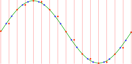
The image below shows a cycle of a sine wave (a ‘pure’ waveform) sampled at regular intervals.
The red lines represent the sampling times, the height of each blue dot is the corresponding sampled value, stored as a number (we have already seen this).
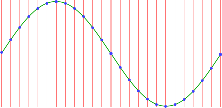
After digitizing it, all that remains of the original wave are the sampled values (the blue dots). However, I will continue drawing the original wave as a visual reference.
Change the time, keep the time
To play this wave at a frequency higher than the original, we can use samples taken farther apart on the original wave.
To play the wave at 1.5x the original frequency, imagine re-reading the (sampled) wave values at 1.5 times the original time interval. I am not referring to the original sampling rate, but to the list of numeric values (the samples).
The points where the red lines here cross the wave represent the new (imaginary) re-sampling points:

But we do not have all these points, so we use the value of the preceding sampling point when a real point (blue dot) is not available.
(it would be much better to linearly interpolate between blue points, but this would cost too much on an 8-bit microcontroller, especially when playing many voices)
The red dots here are the new, resampled values, that is the values we will actually send to the DAC:
Now we take the red dot values and play them out (using the DAC) using the original sampling rate as playing rate. We have produced a wave with 1.5x the original frequency:

As you can see, in the same number of samples as one cycle of the original wave, i.e in the same time because we are using the same playing rate, we play 1.5 wave cycles. So we are playing at 1.5 times the original frequency: a D instead of the original G.
This operation is usually done on the fly, without any precalculation. I will later show some AVR code.
Actually, it is not necessary for the playing rate to be the same as the sampling frequency (in fact, in play-v6 it is not). What really counts to avoid the problems I mentioned above in “The naive way” is that the playing rate is the same for all notes.
The ugly truth
Doesn’t the above resampled wave look nice?
Well, let us remove the nice sine wave drawing and connect the red dots to see how the DAC output will actually look:
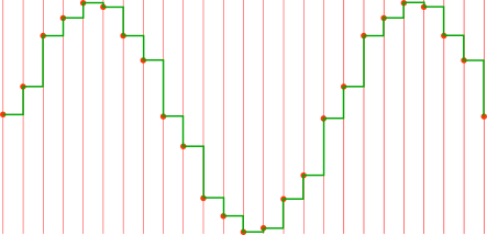
Urgh! Here the lack of interpolation is quite visible as wave asymmetry. Such a sound will surely be totally unacceptable!
Well, actually it could sound pleasant enough. The trick is to have enough sampling points in the original wave to avoid gross distortion, so the original wave should be digitized at the highest possible sampling rate.
That’s why I preferred to shorten the guitar sound, rather than reducing its sampling rate.
So, to recap, we have a sampled guitar string sound and we know (at least in theory) how to play it at different rates to produce different notes.
I previously wrote that optimization is the art of finding the best compromise between conflicting requirements, so in the next post I will consider another set of conflicting requirements.
Squeezing audio samples into Arduino memory
I digitized 6 seconds of a guitar string sound, on a single channel (i.e. monophonic) using a 44.1 kHz sampling rate, so the digitized sound contained:
44100 samples/s * 6 s = 264600 samples
Each sample from my PC audio interface is stored into 16 bits (2 bytes), so the total amount of memory required is:
264600 samples * 2 bytes = 529200 bytes
Ooops, the Arduino Uno microcontroller only has 32 KB of Flash memory… and that has to include the program too!
Not good. A compromise is needed: the art of optimization is about finding the best trade-off among conflicting requirements.
Audio budget cuts
The first obvious thing to do is to reduce the size of a sample: using 8 bits instead of 16 bits halves the required memory. The sound quality will suffer (more on this later) but in a sense it would be fitting for a ‘retro’ project on an 8-bit microcontroller. However:
264600 samples * 1 byte = 264600 bytes
It would still require way too much memory, so I could reduce the sampling rate from 44.1 kHz to 22.05 kHz:
22050 samples/s = 22050 bytes/s * 6 s = 132300 bytes
No way to fit these into the available 32768 bytes (minus the memory used by the program), so I must also reduce the duration of the digitized audio.
Here it is convenient to reason backwards: how much Flash memory can I spare to contain the guitar sound?
The player program will be small, probably a few kilobytes. If I reserve 8 KB for the program, the guitar sound must fit into the remaining 24 KB, i.e. 24576 samples at most.
What would be the duration of a digitized sound made of 24576 samples, played out at 22050 samples/s?
24576 / 22050 = about 1.11 s
I actually chose a sligthly different compromise: I kept the original 44.1 kHz sampling frequency and further halved the playing time:
sampling rate: 44100 Hz
numer of samples: about 24000
duration: about 0.6 s
Keeping a higher sampling frequency, i.e. a more finely defined original signal, helps in reducing undesired effects such as intermodulation distortion (more on this later), in this case at the cost of a shorter sound.
Reshaping a sound with Audacity
I had to shorten the 6-second digitized sound to 0.6-seconds, at the same time trying not to completely lose its timbric quality: I hoped it could still sound like a sort of guitar string.
I opted to build a ‘half-fake’ guitar sound: I kept only the first 0.6 seconds of the original sound, but I reshaped this shorter sound using the Audacity “envelope” tool to get a faster decay, i.e. the decreasing of volume with time:
The net effect of this operation is that the sound is much shorter than the original, but its volume shape (the ‘envelope’) is similar. Also note how I cut off the ending with a final, faster decay when the allotted time is about to expire.
Listen to the reshaped sound:
It sounds more or less like the string of a cheap guitar, whose sound is dampened with a fingertip after a little while. The guitar from which I took the original sound was deeply offended, but it could be worse.
Next time: how to play this sound at different frequencies, to produce the desired notes.
How a PWM DAC works
We have seen that a sound is digitized using a microphone to transform it into an electric signal, then by reading the istantaneous voltage of that signal at regular intervals with an Analog to Digital Converter (ADC), getting a series of numeric values.
The red dots in the image below mark the measurement time (horizontal) and the measured value (vertical).
To reproduce the sound from the recorded numbers, we do the exact opposite: we feed the same values at regular intervals to a Digital to Analog Converter (DAC)
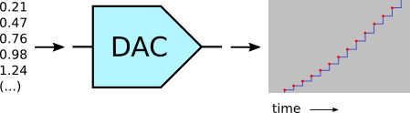
Note that the output voltage, once set, remains constant (horizontal segment) until the next value is converted, producing a staircase-like signal.
The signal will then be smoothed out using an analog “low-pass filter”, but that is not our main concern at the moment.
What worries us (what? You are not worried? You should be!) is that computers can do this because they have both an ADC and a DAC in their audio interface, but the Arduino Uno microcontroller only has an ADC.
But we have to produce an analog audio signal, because our ears are not digital. We need a DAC.
OK, but what is a DAC exactly?
The vertical axis on the above diagrams represents the voltage of the signal, so to recreate the original ‘dots’ we need to produce a precise voltage at regular intervals.
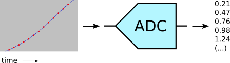
A DAC is exactly that: something that, given a numeric value, produces a voltage proportional to that number.
A hypotetical example:
value     voltage

0.21  ->  0.21 V (volt)

0.47  ->  0.47 V

0.76  ->  0.47 V
If we play out our sequence of numbers at the same frequency used to digitize the sound, i.e. the sampling frequency, the resulting sequence of voltages (filtered to make it smooth) will reproduce the original audio signal.
Cooking dinner with PWM
The ATmega 328P microcontroller used in the Arduino Uno has no DAC, but its hardware can do Pulse-Width Modulation (PWM).
What is PWM? I will cook up an example using my microwave oven; here is its panel:
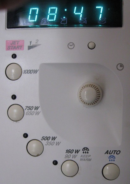
As you can see, it offers different power settings, from 90 W to 1000 W. However, the magnetron tube that makes the microwaves can only produce either 1000 W or nothing.
(I am sure of that: I disassembled and fixed my oven more than once. Last time I replaced a broken spring using a piece of underwear elastic band — but I digress)
If it’s either 1000 W or nothing, how can it produce, say, 500 W?
It uses a simple trick: it turns the magnetron on and off at regular intervals.

The orizontal axis shows time in seconds. It turns on the 1000 W magnetron for six seconds, then turns it off for another six seconds, then repeats this cycle until the cooking time has expired.
It generates 500 W on average by producing 1000 W half of the time (50%).
If I select a power of 750 W, it does this instead:
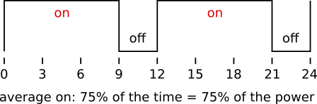
This time the heater, I mean the magnetron, is switched on 75% of the time.
This is PWM: it works by changing the pulse width (the ‘on’ time) within a constant-time cycle, 12 seconds in the case of my oven.
Just for information: the percentage of time the output (the magnetron) stays ‘on’ is called duty cycle. So with a 50% duty cycle I get 500 W, with 75% I get 750 W and with 100% (always on) I obviously get the full 1000 W.
PWM on the Arduino
To cook, er, to generate a variable voltage we can use one of the Arduino PWMs. In the simplest case, they work as 8-bit PWMs.
A basic 8-bit PWM is made with a counter that counts up from 0 to 255. At 0 it turns on a digital output, producing 5 V (volt).
We set a ‘comparator‘ value; when the counter reaches this value, it turns off the output (to 0 V) until the end of the cycle.
When the counter passes 255, it resets to 0 and automatically starts a new cycle, so a full cycle has 256 steps. The horizontal axis here shows the counter value:
Looks similar to the microwave image above? Of course: it’s exactly the same PWM thing!
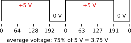
We can control the average output voltage by setting the comparator value:
value  voltage

000 -> 5 V * 1/256   = 0.004 V

127 -> 5 V * 128/256 = 2.5 V

191 -> 5 V * 192/256 = 3.75 V

255 -> 5 V * 256/256 = 5 V
(a technical note: for some of the AVR (Arduino Uno) timer modes we have to write 1 less than the desired value; in any case it would not be possible to use all values between 0 and 256, because those would be 257 values and the counter has a 256-step cycle. In this case we cannot output 0 V; fortunately we can mostly ignore this detail for an audio application)
The exact values are not important here; what counts is that the average output voltage is proportional to the time the output stays on, so the average of the output is our desired voltage: the PWM works as a DAC.
This is done by the hardware: we only have to set the desired output (average) value.
However…
Uh oh, there is some fine print at the bottom of the PWM contract:
- Catch 1: we must average the digital PWM output using an analog filter.
- Catch 2: even after filtering, the PWM cycle frequency could be heard as an audio signal. To prevent this, it should be out of hearing range.
- Catch 3: unwanted sounds (intermodulation products) are generated by the interaction between the PWM frequency and the audio signal. Let’s ignore this for now.
Is that all? Oh no, but that’s all for this post.
Next: squeezing our audio samples into Arduino Flash memory.
Digitizing a guitar string
When I bought an 8-bit Arduino Uno, my first idea was to make a guitar simulator, just for fun (and, to be honest, also to see if I still remembered those skills after so many years).
A guitar has six strings that can play at the same time, so my player needed six independent voices (hence the “play-v6” name for that music engine).
Things didn’t quite play out as I hoped (literally) so I then went on to build a more versatile synth/player.
But the original design was simpler, so I will use it as a starting point.
A digitized sound
My basic idea was to record the sound of a guitar string and to play it out at different frequencies to generate different notes, while (hopefully) retaining some of its quality.
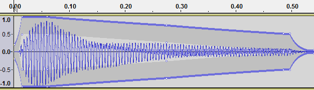
I connected a microphone to the computer, fired up Audacity and plucked a guitar string. Here is what I recorded:

What exactly does this image mean? The horizontal axis represents time (so this is a “time domain diagram”); you can see time displayed above the image, in seconds.
The vertical axis shows the electric signal (technically, the voltage) produced by the microphone; it mirrors the received sound, i.e. the pressure waves in the air created by the string vibration.
The signal has its highest amplitude (sound volume) at about 0.4 seconds, when I plucked the guitar string, then gradually fades out as the sound decreases.
Looking closer
Let’s zoom in to see the same signal in more detail. This shows a much narrower time interval, a bit more than 20 milliseconds (thousandths of a second, abbreviated “ms”):
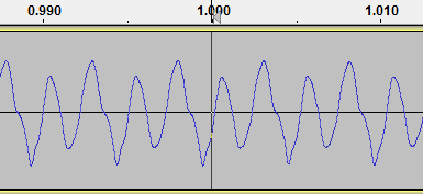
As the time labels show, this image is taken around the 1 second point in the recording (I magnified a bit the vertical axis to better show the details).
Now we can clearly see the signal shape: it reproduces the sound waves created by the oscillation of the guitar string and the resonance of the instrument body.
Notice that the signal tends to repeat itself cyclically, in this case every two peaks.
Measuring the frequency
Zooming further in, this is a single cycle selected in Audacity:
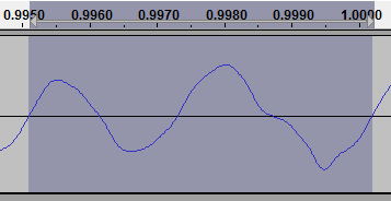
I know, it looks like two distinct waves, but this is the piece of signal that repeats itself periodically, so it is in fact a single cycle of our guitar sound. Real sounds are not as simple as textbook sine waves.
How much time does this single cycle last? That’s easy to estimate; the length of our selection can be seen at the bottom of the window:
![]()
One cycle lasts approximately 0.005 seconds, that is 5 milliseconds.
(this is rather imprecise because the following digits are not shown; for a better measurement we could select 10 cycles and then divide their total length by 10).
How many of these cycles fit in one second, that is in one thousand milliseconds?
1000 ms / 5 ms = 200 cycles
Assuming that 5 ms is correct, we have 200 repetitions per second, that is 200 Hertz (abbreviated “Hz”). This is the approximate frequency of the recorded sound.
In music, the frequency of a sound is called the pitch of a note: different musical notes have different frequencies.
The note I recorded was a G (a Sol in Latin countries) from the third string; its frequency in a well-tuned guitar should be almost exactly 196 Hz, so our measurement looks fairly accurate.
Looking at the samples
Old analog tape recorders did actually record the signal as a continuously variable magnetic field, but the computer is a digital system and cannot do that: it can only store numbers.
It uses instead a device called ADC (Analog to Digital Converter) to measure the istantaneous value of the signal at regular intervals.
It’s like taking note of the room temperature every minute: you can draw a beautiful and rather accurate graph. You are losing some details, but you don’t expect the temperature to change much between a minute and the next (barring a nuclear explosion or such).
So, as long as the signal is measured frequently enough, it could be reproduced without apparent lack of quality.
Zooming in once more on both axes, Audacity shows the measured values, or samples:
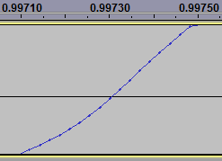
Each dot represents a sample. Its value, the vertical position in the Audacity graph, is what is actually stored (as a number) in the audio file.
Samples are all we have. The dot-connecting lines are just drawn by Audacity for show.
My guitar sound was recorded at 44100 Hz (44.1 kHz), that is 44100 measurements (samples) were taken each second; this is the sampling frequency.
The task ahead
In short, all we have of the original sound is a list of numbers: the sampled values. To reproduce the sound we’ll have to take into account:
- The original frequency of the recorded note (196 Hz).
- The sampling frequency used for the recording (44100 Hz).
- The playing rate we’ll be using on the Arduino.
- The frequency of the note we want to produce. Always playing the same note would be rather boring, wouldn’t it?
It starts getting fun :-)
Next: how a PWM DAC works
8-bit Arduino music synthesis
This series of posts will be both an introduction to (a type of) digital music and a description of the techniques and tricks I used in my play-v6 software music synthesizer.

It will not be a planned route, but rather a sort of Brownian motion around a central theme.
- If you are a beginner, you will find some introductory material on this interdisciplinary field.
- If you are an expert, perhaps you will be interested in some of the more technical descriptions and optimization tricks.
- If you just play with Arduino programming, I hope to shed light on some interesting things.
In short, I aim to please everybody.
That is not possible.
So, this is a failure.
Now that I already failed and therefore I have nothing to lose, I don’t have to worry that something could go wrong. So, let’s start.